
I have recently done a lot of work with matrix transformations, and I found the information on them either sparse, or over-complicated for what I needed. I had to pull together information from many places, split between mathematics focused information, programming reference, and forum posts. So I decided to hopefully write a simple but complete guide on how to understand matrix transformations for the purposes of applying them to computer graphics.
Enter the matrix
When dealing with 2D or 3D graphics programming, there will generally be a couple ways to apply transformations, such as translation (position), rotation, scaling, reflection and skewing (shearing.) There usually is a direct way, with calls to things like setPosition() and setRotation(). However, most frameworks also have another way, using matrix transformations. These are a more powerful way to affect the transformations of the object, and are computationally very quick as they only require addition and multiplication of a few values.
One big advantage is that you can string multiple transformations together one at a time, and they will be applied in the order you add them. To give a practical example, consider the SVG graphics standard for saving vector graphics. SVG files are XML files that use entities such as <rect>, <circle> and <path>. Each of those defines through its attributes how to draw a rectangle, circle, or arbitrary path of lines and curves. Each of those entities can define a "transform" attribute which will contain transformations to apply to the shape right before its drawn. Sometimes it will just be a matrix definition.
So that's simple enough, however the tricky bit comes into play when you consider that SVG also supports a <g> tag, short for "Group." These entities can contain any number of other groups or shapes in them. So you could end up with a deep hierarchy of shapes within groups within groups within groups... Each group can also define a "transform" attribute, to be applied to all groups and shapes within it, and so a shape could have many individual transforms or matrices applied to it. If you were to write an SVG parser (which I did recently and will be posting about soon,) then you would need to be able to concatenate all of those transformations together. With matrices, it's easy.
What are matrices?
A matrix is simply a two dimensional array of numbers. They are used in all kinds of scientific fields. For our purposes we just need to understand how they are defined and how to multiply (concatenate) them together. Matrices in graphics are always defined as \(m \times n\) where \(m\) is the number of rows, and \(n\) is the number of columns. So a \(2 \times 3\) matrix looks like this.
The method in which you access the individual elements of the matrix will vary toolkit to toolkit. One common method, and the one we'll use, is to reference them by \(\text{m}_{mn}\) where 'm' is just the character 'm', '\(m\)' is the row number and '\(n\)' is the column number.
2D and 3D transformations matrices
First, we need to understand what dimensions our matrices are going to be in. Computer graphics generally use matrices of a size \(m \times n\) where each of \(m\) and \(n\) are your dimension size plus one. So if you're working with 2D graphics, then you will be using 3x3 matrices, and 3D graphics use 4x4 matrices. For example, here is a 3x3 matrix used in 2D graphics and a 4x4 matrix used in 3D graphics.
| $$ \begin{bmatrix} \text{m}_{11} & \text{m}_{12} & \text{tx} \\ \text{m}_{21} & \text{m}_{22} & \text{ty} \\ 0 & 0 & 1 \\ \end{bmatrix} $$ | $$ \begin{bmatrix} \text{m}_{11} & \text{m}_{12} & \text{m}_{13} & \text{tx} \\ \text{m}_{21} & \text{m}_{22} & \text{m}_{23} & \text{ty} \\ \text{m}_{31} & \text{m}_{32} & \text{m}_{33} & \text{tz} \\ 0 & 0 & 0 & 1 \\ \end{bmatrix} $$ |
| 3x3 2D Affine Matrix | 4x4 3D Affine Matrix |
|---|
You'll notice that there are a few elements named differently, specifically, tx, ty, and tz. These elements always deal with the translation portion, so it's common to just name them that. For simplicity, we'll be dealing with just 2D 3x3 matrices from here on out, however everything here will also apply for 3D transforms, it's just you have an extra row and column to handle to work on the z-axis.
Homogeneous Matrices
The next thing we need to understand is why we have an extra row in each matrix. Transformation matrices are always "homogeneous." This is so the math is nice and tidy, and allows us to multiply them together and to individual points, which we'll get to later. We don't really need to understand it, thankfully. Just always know that you will have an extra row of zeroes and a one. The transformations we apply with these homogeneous matrices are called "affine transformations."
Identity Matrices
Just a quick note that there exists a matrix that is basically the equivalent of the number \(1\), in that if you multiply a given matrix by an identity matrix, you'll always end up with the given matrix as the result. These identity matrices are used as the foundation of transform matrices, and are the reason the last row is zeroes followed by a one. An identity matrix is always zeroes except a "stripe" of ones going through it diagonally from top left to bottom right.
| $$ \begin{bmatrix} 1 & 0 & 0 \\ 0 & 1 & 0 \\ 0 & 0 & 1 \\ \end{bmatrix} $$ | $$ \begin{bmatrix} 1 & 0 & 0 & 0 \\ 0 & 1 & 0 & 0 \\ 0 & 0 & 1 & 0 \\ 0 & 0 & 0 & 1 \\ \end{bmatrix} $$ |
| 3x3 2D Affine Identity Matrix | 4x4 3D Affine Identity Matrix |
|---|
Multiplication/Concatenation
To go any further we first need to tackle the most complicated part of the new functionality that we're going to need, multiplication. Two matrices can be multiplied together to create a new matrix. The process is a pretty straightforward set of operations, but there are a few rules we have to abide by.
Rule One: Order Matters!
Matrix multiplication is non-commutative, which means that unlike normal numbers, multiplying the matrices \(A \times B\) does not get the same result as \(B \times A\). For this reason, it's often called concatenation instead of multiplication. We'll just call it multiplication from now on. But always remember that the order matters. Generally we take our existing matrix as the operand on the left, and multiply our new matrix as the operand on the right, thus concatenating it onto the end. If it helps, think of it as concatenating strings together. If you were building a sentence one word at a time, you would always concatenate the newest word onto the end of the string as you went, otherwise it would be unreadable. It's basically the same here.
Rule Two: Matrices have to have the same inner dimensions
To multiply two matrices together, their inner dimensions must match. This is best explained by an example.
This is a valid multiplication because the first matrix, A, is a 2x3 matrix, and B is a 3x2 matrix. So their inner dimensions, meaning the number of columns of A (3) is equal to the number of rows of B (3).
An invalid multiplication would look like:
This is because the inner dimensions don't match
And now you know why transformation matrices are always homogeneous. If they didn't have that extra row of zeroes and a one, you wouldn't be able to multiply them together. A 3x3 matrix can always be multiplied by a 3x3 matrix in either direction because their inner dimensions will always match.
Edit: Ok, so that's not the main reason they're homogeneous, just a nice by-product. I'm definitely not a mathematician, but as kyz on reddit pointed out, this excellent explanation was written by one, if you're really curious about the math behind it.
Rule Three: Resulting matrix size
Just a quick note that the resulting matrix after the operation will always be the same number of rows as the left matrix, and the same number of columns as the right matrix. So multiplying our 2x3 matrix by the 3x2 matrix from above will result in a 2x2 matrix. For our purposes, multiplying a 3x3 homogeneous transformation matrix by another will always result in a 3x3 result matrix. Another reason they are always homogeneous!
Multiplication
The actual act of multiplying the two matrices together involves finding the dot-product of each row of the first matrix by each column of the second matrix. As a reminder, a dot-product is where you multiply each element of an array by the corresponding element of a second array, then add the results together. A dot product of two arrays would look like.
With matrix multiplication we just do this multiple times for each element of the final matrix.
Would be
Application
So now that we understand the basics of the matrices we're going to be working with, let's delve into some example code. For this blog I'm going to be using the Gideros framework for a couple reasons. First, it's what I've been using to develop a lot lately, and thus it's what I've been using matrices in, but also because it doesn't have any real built-in matrix functionality. It has a built-in Matrix class, but you can only get and set the matrix of a given sprite. It doesn't have any functionality for manipulating those matrices like most frameworks do. So we're going to write our own.
However, credit is due to ar2rsawseen from the Gideros community for putting together a first draft of matrix functions in his GiderosCodingEasy. His code is where I started, however there were a few issues that prevented them from working properly in what I would consider a normal or standard fashion. He had originally ported that code from an ActionScript project that used matrix transforms in a non-standard way. So I modified his code to work in the same way that I saw in other frameworks. I guess that's what really helped me understand what was going on as I fixed those issues. He has since integrated my changes into his code.
Matrix functionality in Gideros
In Gideros, there is a Sprite class that every visible object is based on, whether it be text, shapes, bitmaps or whatever. This sprite class has a method for getting the current transform matrix, Sprite:getMatrix(), and a method for setting a new transform matrix, Sprite:setMatrix(matrix), which is then applied to the sprite. getMatrix() returns an object of the Matrix class, and setMatrix() takes an object of the Matrix class. The Matrix class itself has many methods for getting and setting the individual elements of the 3x3 matrix, such as getM11(), setM22(), getTx(), setTy(), etc. What it is missing is any mathematical operations, specifically multiplication/concatenation, or any shortcuts to applying transforms, such as translate, rotate, scale or skew. So those are the parts we're going to fill in, and along the way gain a better understanding of how these all work together.
We're going to do this by adding our own methods to the built-in Matrix class. This is possible in Lua because nothing is protected, functions are a first-class type, and almost everything is a table (dictionary hash/array.) Matrix is just a table in the global namespace, with methods as keys and the actual functions as values. So we can just define our own methods like so.
function Matrix:newMethod(var1, var2)
  -- 'self' is automatically defined because we used the lua ':' syntactic sugar
  print("Matrix:newMethod called", self, var1, var2)
end
Once our code is included in a project, you won't be able to tell that newMethod wasn't always there.
Multiplication Method
So our first and probably most important extension to the Matrix class will be a multiply() method that takes a matrix as its argument and multiplies itself by that matrix using the formula we discussed above. We can skip the parts of the dot product that always add a 0 to avoid unnecessary calculations.
function Matrix:multiply(matrix)
  local m11 = self:getM11()*matrix:getM11() + self:getM12()*matrix:getM21()
  local m12 = self:getM11()*matrix:getM12() + self:getM12()*matrix:getM22()
  local m21 = self:getM21()*matrix:getM11() + self:getM22()*matrix:getM21()
  local m22 = self:getM21()*matrix:getM12() + self:getM22()*matrix:getM22()
  local tx  = self:getM11()*matrix:getTx()  + self:getM12()*matrix:getTy() + self:getTx()
  local ty  = self:getM21()*matrix:getTx()  + self:getM22()*matrix:getTy() + self:getTy()
  return self:setElements(m11, m12, m21, m22, tx, ty)
end
This is now our foundation upon which we can build everything else. Please note that Gideros Matrix methods take the arguments in a slightly odd order: m11, m12, m21, m22, tx, ty.
Translation Method
Translation is the simplest matrix to apply. Given a tx and ty as distance to translate x and y by, we simply build the following matrix based on an identity matrix, then multiply it.
This is what our translate() method will look like.
function Matrix:translate(x,y)
  return self:multiply(Matrix.new(1, 0, 0, 1, x, y or x))
end
Scaling Method
Scaling is also pretty simple. Given sx and sy as the amount to scale x and y by, we build the following matrix based on an identity matrix, then multiply it.
And here is the code that will do that.
function Matrix:scale(sx,sy)
  return self:multiply(Matrix.new(sx, 0, 0, sy or sx, 0, 0))
end
Rotation Method
Rotation is a little more involved, but still isn't bad. Given the angle a in radians, our rotation translation matrix looks like this.
Since Gideros functions always deal in degrees and not radians, we'll write our function to take the angle in degrees, then convert to radians for building the matrix.
function Matrix:rotate(deg)
  local rad = math.rad(deg)
  return self:multiply(Matrix.new(math.cos(rad), -math.sin(rad), math.sin(rad), math.cos(rad), 0, 0))
end
Skew Method
Skew is similar to rotation. Given an angle ax to skew on the x-axis, and an angle ay to skew on the y-axis, we construct the matrix as such.
Similar to rotation, we'll take our arguments in degrees and convert to radians for the calculation.
function Matrix:skew(xAng,yAng)
  xAng = math.rad(xAng)
  yAng = math.rad(yAng or xAng)
  return self:multiply(Matrix.new(1, math.tan(xAng), math.tan(yAng), 1, 0, 0))
end
Reflection
Reflecting on the x or y axis is as simple as applying a negative scale in either direction.
-- Flip or mirror on the horizontal axis.
matrix:setScaleX(-1)
Applying a transformation matrix to an arbitrary point
Lastly, it comes in handy every once in a while to be able to apply a given transformation matrix to a single point. This is mainly used to translate between an original coordinate space and the transformed coordinate space. Points can be represented as a 3x1 matrix.
This means we can multiply a 3x3 transformation matrix times a point, but not the other way, since the inner products wouldn't match. So this multiplication simply looks like this.
Converting this formula to code will result in this method.
function Matrix:applyToPoint(x, y)
  local newX = self:getM11() * x + self:getM12() * y + self:getTx()
  local newY = self:getM21() * x + self:getM22() * y + self:getTy()
  return newX, newY
end
Putting it all together
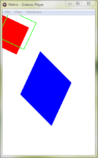
Once this is all in place, the following example code is an idea of what is possible.
-- Create a rectangle Shape which inherits from Sprite sized 100 pixels wide and 100 pixels tall
local box = createBox(100,100)

-- Set a new position for the box.
box:setPosition(100,200)

-- This gets the current matrix, which includes the new position we just set
local matrix = box:getMatrix()

-- Move to our new anchor point relative to current position
matrix:translate(50,50)

-- Rotate by 45 degrees
matrix:rotate(45)

-- Scale by 150%
matrix:scale(1.5)

-- Skew the x axis by 20 degrees
matrix:skew(20, 0)

-- Put it back
matrix:translate(-50,-50)

-- Apply our new concatenated transform to the sprite
box:setMatrix(matrix)
Full code and Sample project
I have made the full code to this Matrix extension available on Github. You can view just the Matrix class extensions or a full example Gideros project that shows the code in action. The code is the same as in this post, plus a few extra convenience methods.
References
I'd like to thank the following wonderful references that I read when I was learning all of this.
- Wikipedia: Matrix (mathematics)
- Wikipedia: Transformation matrix
- 2D Transformations
- Gideros Mobile Framework
- ar2rsawseen's GiderosCodingEasy
- W3C SVG Standards section on transformations
- Microsoft XNA Library - Matrix class
- Apple CGAffineTransform Reference
- Many posts on StackOverflow.com
- Matrices in HTML Applet - How I generated the HTML for my matrices
Real world uses
I'll soon post followups to this post showing a couple examples of how I used this new Matrix class to implement a movable anchor for Gideros Sprites, and to parse SVG files and all their transforms. For example, here's my AnchorSprite implementation, which supports moving the anchor for a sprite from [0,0] to anywhere you want, and affects all position, rotation, scale and skew operations.
![]()
More on 3D
When applying these same techniques to 3D, most of the basics are the same, however you have bigger matrices and one more axis to handle. Matrix multiplication still works the same, the matrices are still homogeneous, identity matrices are the same. What will be different are the types of matrices you construct to do your transformations. Here is just a quick list of these matrices.
| $$ \begin{bmatrix} 1 & 0 & 0 & tx \\ 0 & 1 & 0 & ty \\ 0 & 0 & 1 & tz \\ 0 & 0 & 0 & 1 \\ \end{bmatrix} $$ | $$ \begin{bmatrix} sx & 0 & 0 & 0 \\ 0 & sy & 0 & 0 \\ 0 & 0 & sz & 0 \\ 0 & 0 & 0 & 1 \\ \end{bmatrix} $$ |
| 4x4 3D Translation Matrix | 4x4 3D Scale Matrix |
|---|
| $$ \begin{bmatrix} 1 & 0 & 0 & 0 \\ 0 & \cos(a) & -\sin(a) & 0 \\ 0 & \sin(a) & \cos(a) & 0 \\ 0 & 0 & 0 & 1 \\ \end{bmatrix} $$ | $$ \begin{bmatrix} \cos(a) & 0 & \sin(a) & 0 \\ 0 & 1 & 0 & 0 \\ -\sin(a) & 0 & \cos(a) & 0 \\ 0 & 0 & 0 & 1 \\ \end{bmatrix} $$ | $$ \begin{bmatrix} \cos(a) & -\sin(a) & 0 & 0 \\ \sin(a) & \cos(a) & 0 & 0 \\ 0 & 0 & 1 & 0 \\ 0 & 0 & 0 & 1 \\ \end{bmatrix} $$ |
| 4x4 3D x-axis Rotation Matrix | 4x4 3D y-axis Rotation Matrix | 4x4 3D z-axis Rotation Matrix |
|---|
| $$ \begin{bmatrix} 1 & 0 & 0 & 0 \\ \tan(a) & 1 & 0 & 0 \\ 0 & 0 & 1 & 0 \\ 0 & 0 & 0 & 1 \\ \end{bmatrix} $$ | $$ \begin{bmatrix} 1 & 0 & 0 & 0 \\ 0 & 1 & 0 & 0 \\ \tan(a) & 0 & 1 & 0 \\ 0 & 0 & 0 & 1 \\ \end{bmatrix} $$ | $$ \begin{bmatrix} 1 & \tan(a) & 0 & 0 \\ 0 & 1 & 0 & 0 \\ 0 & 0 & 1 & 0 \\ 0 & 0 & 0 & 1 \\ \end{bmatrix} $$ |
| 4x4 3D xz-axis Skew Matrix | 4x4 3D zx-axis Skew Matrix | 4x4 3D yz-axis Skew Matrix |
|---|
| $$ \begin{bmatrix} 1 & 0 & 0 & 0 \\ 0 & 1 & 0 & 0 \\ 0 & \tan(a) & 1 & 0 \\ 0 & 0 & 0 & 1 \\ \end{bmatrix} $$ | $$ \begin{bmatrix} 1 & 0 & \tan(a) & 0 \\ 0 & 1 & 0 & 0 \\ 0 & 0 & 1 & 0 \\ 0 & 0 & 0 & 1 \\ \end{bmatrix} $$ | $$ \begin{bmatrix} 1 & 0 & 0 & 0 \\ 0 & 1 & \tan(a) & 0 \\ 0 & 0 & 1 & 0 \\ 0 & 0 & 0 & 1 \\ \end{bmatrix} $$ |
| 4x4 3D zy-axis Skew Matrix | 4x4 3D xy-axis Skew Matrix | 4x4 3D yx-axis Skew Matrix |
|---|
Points in 3D are a 4x1 of \([x,y,z,1]^T\), and the math to apply them to a transform is the same as above, just one more axis to determine. Here are some further resources specific to 3D transformations.